Given a function that models a certain phenomenon, it’s natural to ask such questions as “how is the function changing on a given interval” or “on which interval is the function changing more rapidly?” The concept of average rate of change enables us to make these questions more mathematically precise. Initially, we will focus on the average rate of change of an object moving along a straight-line path.
For a function \(s\) that tells the location of a moving object along a straight path at time \(t\text{,}\) we define the average rate of change of \(s\) on the interval \([a,b]\) to be the quantity
Let the height function for a ball tossed vertically be given by \(s(t) = 64 - 16(t-1)^2\text{,}\) where \(t\) is measured in seconds and \(s\) is measured in feet above the ground.
In Desmos, plot the function \(s(t) = 64 - 16(t-1)^2\) along with the points \((1.5,s(1.5))\) and \((2.5, s(2.5))\text{.}\) Make a copy of your plot on the axes in the figure provided, labeling key points as well as the scale on your axes. What is the domain of the model? The range? Why?
Work by hand to find the equation of the line through the points \((1.5,s(1.5))\) and \((2.5, s(2.5))\text{.}\) Write the line in the form \(y = mt + b\) and plot the line in Desmos, as well as on the axes above.
How do your answers in the preceding questions change if we instead consider the interval \([0.25, 0.75]\text{?}\)\([0.5, 1.5]\text{?}\)\([1,3]\text{?}\)
Subsection1.3.2Defining and interpreting the average rate of change of a function
In the context of a function that measures height or position of a moving object at a given time, the meaning of the average rate of change of the function on a given interval is the average velocity of the moving object because it is the ratio of change in position to change in time. For example, in Preview Activity 1.3.1, the units on \(AV_{[1.5,2.5]} = -32\) are “feet per second” since the units on the numerator are “feet” and on the denominator “seconds”. Morever, \(-32\) is numerically the same value as the slope of the line that connects the two corresponding points on the graph of the position function, as seen in Figure 1.3.1. The fact that the average rate of change is negative in this example indicates that the ball is falling.
While the average rate of change of a position function tells us the moving object’s average velocity, in other contexts, the average rate of change of a function can be similarly defined and has a related interpretation. We make the following formal definition.
In every situation, the units on the average rate of change help us interpret its meaning, and those units are always “units of output per unit of input.” Moreover, the average rate of change of \(f\) on \([a,b]\) always corresponds to the slope of the line between the points \((a,f(a))\) and \((b,f(b))\text{,}\) as seen in Figure 1.3.2.
According to the US census, the populations of Kent and Ottawa Counties in Michigan where GVSU is located (Grand Rapids is in Kent, Allendale in Ottawa) from 1960 to 2010 measured in \(10\)-year intervals are given in the following tables.
Write a careful sentence that explains the meaning of the average rate of change of the Ottawa county population on the time interval \([1990,2010]\text{.}\) Your sentence should begin something like “In an average year between 1990 and 2010, the population of Ottawa County was \(\ldots\)”
Which county had a greater average rate of change during the time interval \([2000,2010]\text{?}\) Were there any intervals in which one of the counties had a negative average rate of change?
The average rate of change of a function on an interval gives us an excellent way to describe how the function behaves, on average. For instance, if we compute \(AV_{[1970,2000]}\) for Kent County, we find that
which tells us that in an average year from 1970 to 2000, the population of Kent County increased by about \(5443\) people. Said differently, we could also say that from 1970 to 2000, Kent County was growing at an average rate of \(5443\) people per year. These ideas also afford the opportunity to make comparisons over time. Since
we can not only say that Kent county’s population increased by about \(7370\) in an average year between 1990 and 2000, but also that the population was growing faster from 1990 to 2000 than it did from 1970 to 2000.
Finally, we can even use the average rate of change of a function to predict future behavior. Since the population was changing on average by \(7370.5\) people per year from 1990 to 2000, we can estimate that the population in 2002 is
Subsection1.3.3How average rate of change indicates function trends
We have already seen that it is natural to use words such as “increasing” and “decreasing” to describe a function’s behavior. For instance, for the tennis ball whose height is modeled by \(s(t) = 64 - 16(t-1)^2\text{,}\) we computed that \(AV_{[1.5,2.5]} = -32\text{,}\) which indicates that on the interval \([1.5,2.5]\text{,}\) the tennis ball’s height is decreasing at an average rate of \(32\) feet per second. Similarly, for the population of Kent County, since \(AV_{[1990,2000]} = 7370.5\text{,}\) we know that on the interval \([1990,2000]\) the population is increasing at an average rate of \(7370.5\) people per year.
Let \(f\) be a function defined on an interval \((a,b)\) (that is, on the set of all \(x\) for which \(a \lt x \lt b\)). We say that \(f\) is increasing on \((a,b)\) provided that the function is always rising as we move from left to right. That is, for any \(x\) and \(y\) in \((a,b)\text{,}\) if \(x \lt y\text{,}\) then \(f(x) \lt f(y)\text{.}\)
Similarly, we say that \(f\) is decreasing on \((a,b)\) provided that the function is always falling as we move from left to right. That is, for any \(x\) and \(y\) in \((a,b)\text{,}\) if \(x \lt y\text{,}\) then \(f(x) \gt f(y)\text{.}\)
If we compute the average rate of change of a function on an interval, we can decide if the function is increasing or decreasing on average on the interval, but it takes more work 1
Calculus offers one way to justify that a function is always increasing or always decreasing on an interval.
to decide if the function is increasing or decreasing always on the interval.
Let’s consider two different functions and see how different computations of their average rate of change tells us about their respective behavior. Plots of \(q\) and \(h\) are shown in the figures in part (c).
Consider the function \(q(x) = 4-(x-2)^2\text{.}\) Compute \(AV_{[0,1]}\text{,}\)\(AV_{[1,2]}\text{,}\)\(AV_{[2,3]}\text{,}\) and \(AV_{[3,4]}\text{.}\) What do your last two computations tell you about the behavior of the function \(q\) on \([2,4]\text{?}\)
Consider the function \(h(t) = 3 - 2(0.5)^t\text{.}\) Compute \(AV_{[-1,1]}\text{,}\)\(AV_{[1,3]}\text{,}\) and \(AV_{[3,5]}\text{.}\) What do your computations tell you about the behavior of the function \(h\) on \([-1,5]\text{?}\)
On the graphs that follow (\(q\) at left, \(h\) at right), plot the line segments whose respective slopes are the average rates of change you computed in (a) and (b).
Give an example of a function that has the same average rate of change no matter what interval you choose. You can provide your example through a table, a graph, or a formula; regardless of your choice, write a sentence to explain.
It is helpful be able to connect information about a function’s average rate of change and its graph. For instance, if we have determined that \(AV_{[-3,2]} = 1.75\) for some function \(f\text{,}\) this tells us that, on average, the function rises between the points \(x = -3\) and \(x = 2\) and does so at an average rate of \(1.75\) vertical units for every horizontal unit. Moreover, we can even determine that the difference between \(f(2)\) and \(f(-3)\) is
Sketch at least two different possible graphs that satisfy the criteria for the function stated in each part. Make your graphs as significantly different as you can. If it is impossible for a graph to satisfy the criteria, explain why.
\(g\) is a function defined on \([-1,7]\) such that \(g(4) = 3\text{,}\)\(AV_{[0,4]} = 0.5\text{,}\) and \(g\) is not always increasing on \((0,4)\text{.}\)
The value of \(AV_{[a,b]} = \frac{f(b) - f(a)}{b-a}\) tells us how much the function rises or falls, on average, for each additional unit we move to the right on the graph. For instance, if \(AV_{[3,7]} = 0.75\text{,}\) this means that for additional \(1\)-unit increase in the value of \(x\) on the interval \([3,7]\text{,}\) the function increases, on average, by \(0.75\) units. In applied settings, the units of \(AV_{[a,b]}\) are “units of output per unit of input”.
The value of \(AV_{[a,b]} = \frac{f(b) - f(a)}{b-a}\) is also the slope of the line that passes through the points \((a,f(a))\) and \((b,f(b))\) on the graph of \(f\text{,}\) as shown in Figure 1.3.2.
Let \(P_1\) and \(P_2\) be the populations (in hundreds) of Town 1 and Town 2, respectively. The table below shows data for these two populations for five different years.
(a) From 1980 to 1987, the average rate of change of the population of Town 1 was hundred people per year, and the average rate of change of the population of Town 2 was hundred people per year.
(b) From 1987 to 1999, the average rate of change of the population of Town 1 was hundred people per year, and the average rate of change of the population of Town 2 was hundred people per year.
(c) From 1980 to 1999, the average rate of change of the population of Town 1 was hundred people per year, and the average rate of change of the population of Town 2 was hundred people per year.
In 2005, you have 45 CDs in your collection. In 2008, you have 130 CDs. In 2012, you have 50 CDs. What is the average rate of change in the size of your CD collection between:
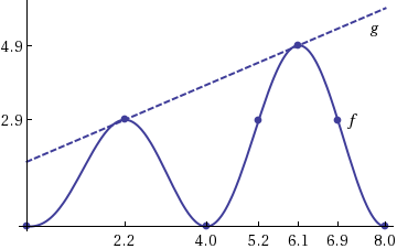
Function \(f\) starts at the origin, goes up and back down to the x-axis and then up higher and then back down to the axis again, with the two peaks at \(x=2.2\) and \(x=6.1\text{.}\) It hits the x-axis at \(x=0\text{,}\)\(x=4\text{,}\) and \(x=8\text{.}\) Function \(g\) is an increasing line going though the points occuring at the two peaks of \(f\text{,}\) that is, \((2.2, f(2.2))\) and \((6.1,f(6.1))\text{.}\)
a) For each of the intervals, find the values of \(\Delta D\) and \(\Delta t\) between the indicated start and end times. Enter your answers in their respective columns in the table below.
b) Based on your results from (a) it follows that the average rate of change of \(D\) is constant, it does not depend over which interval of time you choose. What is the constant rate of change of \(D\text{?}\)
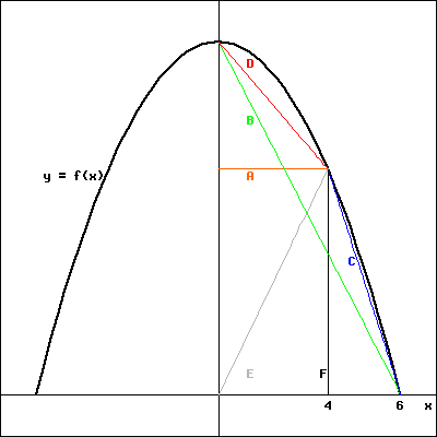
b) Based on the graph sketched below, match each of your answers in (i) - (iii) with one of the lines labeled A - F. Type the corresponding letter of the line segment next to the appropriate formula. Clearly not all letters will be used.
A cold can of soda is removed from a refrigerator. Its temperature \(F\) in degrees Fahrenheit is measured at \(5\)-minute intervals, as recorded in the following table.
Determine \(AV_{[0,5]}\text{,}\)\(AV_{[5,10]}\text{,}\) and \(AV_{[10,15]}\text{,}\) including appropriate units. Choose one of these quantities and write a careful sentence to explain its meaning. Your sentence might look something like “On the interval \(\ldots\text{,}\) the temperature of the soda is \(\ldots\) on average by \(\ldots\) for each \(1\)-unit increase in \(\ldots\)”.
The position of a car driving along a straight road at time \(t\) in minutes is given by the function \(y = s(t)\) that is pictured in Figure 1.3.6. The car’s position function has units measured in thousands of feet. For instance, the point \((2,4)\) on the graph indicates that after 2 minutes, the car has traveled 4000 feet.
Figure1.3.6.The graph of \(y = s(t)\text{,}\) the position of the car (measured in thousands of feet from its starting location) at time \(t\) in minutes.
In everyday language, describe the behavior of the car over the provided time interval. In particular, carefully discuss what is happening on each of the time intervals \([0,1]\text{,}\)\([1,2]\text{,}\)\([2,3]\text{,}\)\([3,4]\text{,}\) and \([4,5]\text{,}\) plus provide commentary overall on what the car is doing on the interval \([0,12]\text{.}\)
Compute the average rate of change of \(s\) on the intervals \([3,4]\text{,}\)\([4,6]\text{,}\) and \([5,8]\text{.}\) Label your results using the notation “\(AV_{[a,b]}\)” appropriately, and include units on each quantity.
On the graph of \(s\text{,}\) sketch the three lines whose slope corresponds to the values of \(AV_{[3,4]}\text{,}\)\(AV_{[4,6]}\text{,}\) and \(AV_{[5,8]}\) that you computed in (b).
Consider an inverted conical tank (point down) whose top has a radius of \(3\) feet and that is \(2\) feet deep. The tank is initially empty and then is filled at a constant rate of \(0.75\) cubic feet per minute. Let \(V=f(t)\) denote the volume of water (in cubic feet) at time \(t\) in minutes, and let \(h= g(t)\) denote the depth of the water (in feet) at time \(t\text{.}\) It turns out that the formula for the function \(g\) is \(g(t) = \left( \frac{t}{\pi} \right)^{1/3}\text{.}\)
For the height function \(h = g(t) = \left( \frac{t}{\pi} \right)^{1/3}\text{,}\) compute \(AV_{[0,2]}\text{,}\)\(AV_{[2,4]}\text{,}\) and \(AV_{[4,6]}\text{.}\) Include units on your results.
Again working with the height function, can you determine an interval \([a,b]\) on which \(AV_{[a,b]} = 2\) feet per minute? If yes, state the interval; if not, explain why there is no such interval.
Now consider the volume function, \(V = f(t)\text{.}\) Even though we don’t have a formula for \(f\text{,}\) is it possible to determine the average rate of change of the volume function on the intervals \([0,2]\text{,}\)\([2,4]\text{,}\) and \([4,6]\text{?}\) Why or why not?