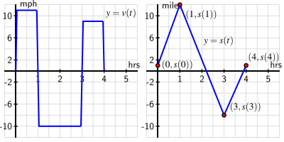
The average velocities are negative; the instantaneous velocity was positive. Downward motion corresponds to negative average velocity; upward motion to positive average velocity.
\(AV_{[2.45,7]} \approx \frac{-3.5-0}{7-2.45}=\frac{-3.5}{4.55}=-0.7692\) m/sec. The average velocity is not the same on every time interval within \([2.45,7]\text{.}\)
When the diver is going upward, her velocity is positive. When she is going downward, her velocity is negative. At the peak of her dive and when her feet touch the bottom of the pool.
It looks like when the position function is steep, the velocity function’s value is farther away from zero, and that whenever the height/position function is rising/increasing, the velocity function has a positive value. Similarly, whenever the position function is decreasing, the velocity is negative.
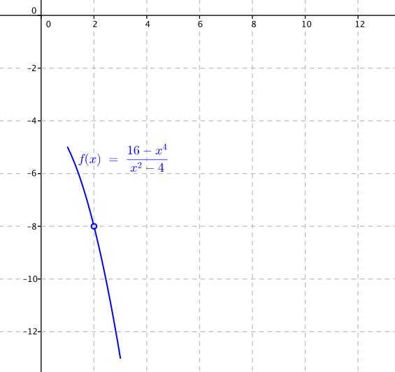
A plot of the function \(f(x) = \frac{16-x^4}{x^2-4}\) on the interval \(1 \lt x \lt 3\text{.}\) The graph looks like a parabola that is decreasing from the point \((1,-5)\) to \((3,-13)\text{,}\) except there’s a small open circle at the point \((2,-8)\text{,}\) which indicates that \(f(2)\) is not defined.
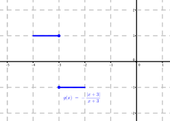
For \(-4 \lt x \lt -3\text{,}\)\(g(x) = 1\text{,}\) while for \(-3 \lt x \lt -2\text{,}\)\(g(x) = -1\text{,}\) which shows that there’s a jump in the graph of \(g\) at \(x = -3\text{,}\) along with the fact that \(g(-3)\) is not defined
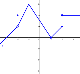
One possible graph of a function \(f(x)\) that satisfies the given conditions. At \(x = -2\text{,}\) the function has a small open circle on the graph at the point \((-2,1)\) and a small filled circle at \((-2,2)\) to indicate that \(f(-2) = 2\) and \(\lim_{x \to -2} f(x) = 1\text{.}\) The graph passes through \((-1,3)\) with no jumps or holes to satisfy \(f(-1) = 3\) and \(\lim_{x \to -1} f(x) = 3\text{.}\) The graph has a small open circle at \((1,0)\) to show that \(f(1)\) is not defined and \(\lim_{x \to 1} f(x) = 0\text{.}\) And finally, the graph jumps from a height of \(f(2) = 1\) to a height of \(y = 2\) for \(x \gt 2\) to have \(\lim_{x \to 2} f(x)\) not exist.
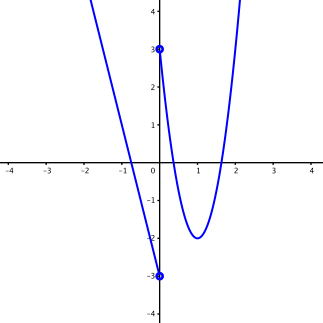
One possible graph of a function \(g(x)\) that satisfies the given conditions. In particular, the graph passes through the points \((-2,3)\text{,}\)\((-1,-1)\text{,}\)\((1,-2)\text{,}\) and \((2,3)\text{.}\) To the left of \(x = 0\text{,}\) the graph is a line with negative slope that passes through \((-2,3)\) and \((0,-3)\) with a small open circle at \((0,-3)\text{.}\) To the right of \(x = 0\text{,}\) the graph is a parabola with \(y\)-intercept at \((0,3)\) (but a small open circle there) and a vertex at \((1,-2)\text{.}\)
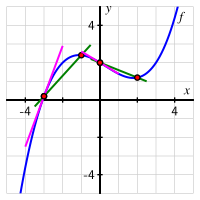
The points identified on the graph are \((-3,f(-3))\text{,}\)\((-1,f(-1))\text{,}\)\((0,f(0))\text{,}\) and \((2,f(2))\text{.}\) The first secant line shown passes through \((-3,f(-3))\) and \((-1,f(-1))\text{,}\) and the second secant line passes through \((0,f(0))\) and \((2,f(2))\text{.}\) Finally, there is a tangent line to the curve at \((-3,f(-3))\) and another tangent line to the curve at \((0,f(0))\text{.}\)
For instance, you could let \(f(-3) = 3\) and have \(f\) pass through the points \((-3,3)\text{,}\)\((-1,-2)\text{,}\)\((0,-3)\text{,}\)\((1,-2)\text{,}\) and \((3,-1)\) and draw the desired tangent lines accordingly.
For instance, you could draw a function \(g\) that passes through the points \((-2,3)\text{,}\)\((-1,2)\text{,}\)\((1,0)\text{,}\)\((2,0)\text{,}\) and \((3,3)\) in such a way that the tangent line at \((-1,2)\) is horizontal and the tangent line at \((2,0)\) has slope \(1\text{.}\)
\(AV_{[0,7]}=\frac{0.1175}{7} \approx 0.01679\) billion people per year; \(P'(7) \approx 0.1762\) billion people per year; \(P'(7) \gt AV_{[0,7]}\text{.}\)
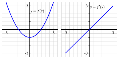
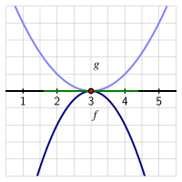
At left, one possible graph for \(f\text{:}\) a quadratic function that opens upward, is shifted down \(1\) unit, and that has the requisite slopes described in the exercise. At right, a possible corresponding graph of \(f'\text{:}\) a linear function that has slope \(m=1\) and that passes through \((0,0)\text{.}\)
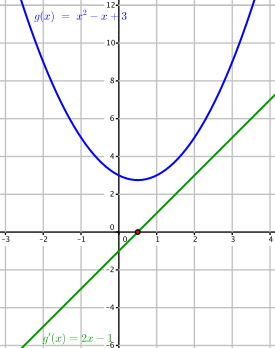
A plot of the original quadratic function \(g(x) = x^2 - x + 3\) along with its derivative, \(g'(x) = 2x - 1\text{.}\) In the graph, we notice how \(g'(x)\) crosses the \(x\)-axis at the same location where \(g(x)\) has a horizontal tangent line.
The constants \(3\) and \(12\) don’t seem to affect the results at all. The coefficient \(-4\) on the linear term in \(p(x)\) appears to make the “\(-4\)” appear in \(p'(x)= 10x - 4\text{.}\) The leading coefficient \(5\) in \((x) = 5x^2 - 4x + 12\) leads to the coefficient of “\(10\)” in \(p'(x) = 10x -4\text{.}\)
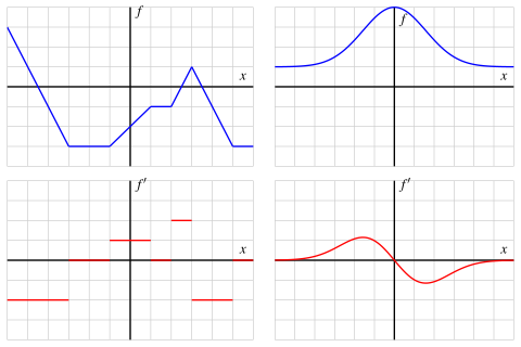
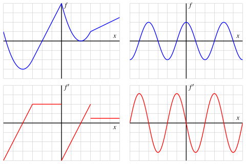
This image consists of \(4\) sets of axes arranged in two rows and two columns. There is no scale on any of the axes. In the top left, there is a function \(f\) that is piecewise linear, consisting of line segments that connect the following points: \((-6,3)\text{,}\)\((-3,-3)\text{,}\)\((1,-1)\text{,}\)\((2,-1)\text{,}\)\((3,1)\text{,}\)\((5,-3)\text{,}\) and \((6,-3)\text{.}\) In the top right, there is a different function, also labeled \(f\) that looks like the normal distribution (i.e., a bell curve), with its maximum at the point \((0,4)\) and a horizontal asymptote in each direction at \(y = 1\text{.}\)
Beneath each of these two figures given figures are plots of their derivative. On the left, the derivative function is piecewise constant. For example, its value on the interval \((-6,-3)\) is \(f'(x) = -2\text{,}\) which is the slope of the corresponding line segment on the graph of \(f(x)\text{.}\) On the right, the derivative function is positive for \(x \lt 0\text{,}\) negative for \(x \gt 0\text{,}\) passes through \((0,0)\text{,}\) and approaches its horizontal asymptote of \(y = 0\) as \(x\) both decreases and increases without bound. The most extreme values of \(f'(x)\) occur at the approximate points \((-1.5,1.1)\) and \((1.5,-1.1)\text{.}\)
This image consists of \(4\) sets of axes arranged in two rows and two columns. There is no scale on any of the axes. In the top left, there is a function \(f\) that is piecewise-defined, consisting of pieces that are quadratic or linear. The first piece is a quadratic function that passes through \((-6,1)\text{,}\)\((-4,-3)\) (the vertex), and \((-3,-2)\text{;}\) the next piece is a line segment from \((-3,-2)\) to \((0,4)\text{;}\) the third piece is a quadratic function through \((0,4)\text{,}\)\((2,0)\) (the vertex), and \((3,1)\text{.}\) The final piece is a line segment through \((3,1)\) and \((6,2.5)\text{.}\) In the top right, there is a different function, also labeled \(f\) that looks like the cosine function: one period of this curve has the function passing through the points \((0,2)\text{,}\)\((1,0)\text{,}\)\((2,-2)\text{,}\)\((3,0)\text{,}\) and \((4,2)\text{.}\)
Beneath each of these two figures are plots of their respective derivatives. On the left, \(f'(x)\) is a piecewise linear function: where \(f(x)\) is quadratic, \(f'(x)\) is linear, and where \(f(x)\) is linear, \(f'(x)\) is constant. For example, on the interval \(0 \lt x \lt 3\text{,}\)\(f'(x)\) is given by the line segment passing through \((0,-4)\) and \((3,2)\text{;}\) on the interval \(3 \lt x \lt 6\text{,}\)\(f'(x)\) is given by the horizontal line segment passing through \((3,0.5)\) and \((6,0.5)\text{.}\) Note that \(f'(3)\) is not defined.
On the right, the derivative graph looks like a stretched version of the negative sine function. One period of this graph passes through the following points: \((0,0)\text{,}\)\((1,-3)\text{,}\)\((2,0)\text{,}\)\((3,3)\text{,}\) and \((4,0)\text{.}\)
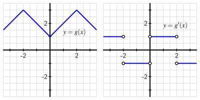
Two adjacent coordinate axes where each grid has \(x\) ranging horizontally from \(-3.5\) to \(-3.5\text{,}\) and \(y\) ranging vertically from \(-3.5\) to \(-3.5\text{.}\) On the righthand axes, a plot of the piecewise constant function \(g'(x)\) is shown, which has the value \(g'(x) = 2\) on the intervals \(-3.5 \lt x \lt -2\) and \(0 \lt x \lt 2\text{,}\) and has the value \(g'(x) = -2\) on the intervals \(-2 \lt x \lt 0\) and \(2 \lt x \lt 3.5\text{.}\)
On the lefthand axes, we see a plot of the continuous function \(g(x)\) whose derivative is \(g'(x)\text{.}\) The pictured function is piecewise linear and passes through the points \((-3.5,1.5)\text{,}\)\((-2,3)\text{,}\)\((0,1)\text{,}\)\((2,3)\text{,}\) and \((3.5,1.5)\text{.}\)
For a patient taking a \(50\) ml dose, adding one more ml to the dose leads us to expect a temperature change that is about \(0.02\) degrees less than the temperature change induced by a \(50\) ml dose.
The graph of \(h\) might have the general shape of the graph of \(y = e^{-x}\) for positive values of \(x\text{:}\) always positive, always decreasing, and bending upwards while tending to \(0\) as \(x\) increases.
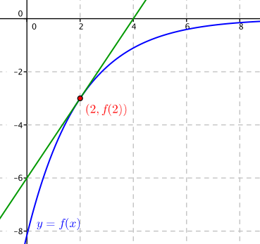
A plot of a function \(f\) with the properties that \(f(2) = -3\text{,}\)\(f'(2) = 1.5\text{,}\)\(f''(2) = -0.25\text{;}\) a plot of the tangent line to the curve at \((2,-3)\) is also shown. The graph of this particular example function \(f\) is always increasing and concave up, and shown for an interval of \(0 \lt x \lt 8\) and \(-8 \lt y \lt 0\text{.}\)
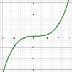
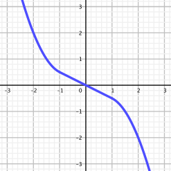
A graph that meets the stated criteria of the exercise. This function looks like \(f(x) = -x^3\) provided that \(x \lt -1\) or \(x \gt 1\text{.}\) On the interval \(-1 \le x \le 1\text{,}\) the function is a straight line that joins the two cubic-looking parts.
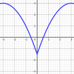
A graph that meets the stated criteria of the exercise. This function looks like two downward-opening parabolas that meet at a corner point at \((0,-1.5)\text{.}\) The left parabola has its vertex at \((-3,3)\text{;}\) the right parabola has its vertex at \((3,3)\text{.}\)
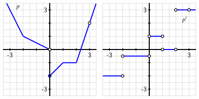
At left, the piecewise linear function \(y = p(x)\) that consists of \(5\) pieces, the line segments that connect \((-3.25,3.5)\) and \((-2,1)\text{;}\)\((-2,3.1)\) and \((0,0)\text{;}\)\((0,-2)\) and \((1,-1)\text{;}\)\((1,-1)\) and \((2,-1)\text{;}\) and \((2,-1)\) and \((3.5,3.5)\text{.}\) In addition, there are open circles at \((0,0)\) and \((3,2)\text{,}\) as well as a filled circle at \((0,-2)\text{.}\)
At right, the piecewise constant function \(y = p'(x)\text{.}\) On the corresponding intervals that align with the piecewise function \(y = p(x)\text{,}\) the value of \(p'(x)\) is, respectively, \(-2\text{,}\)\(-\frac{1}{2}\text{,}\)\(1\text{,}\)\(0\text{,}\) and \(3\text{.}\) Note that each “step” of the function \(y = p'(x)\) has open circles at each end since \(p'(x)\) is undefined at the corner points (and jumps) of \(p(x)\text{.}\) For example, there’s a line segment on the graph of \(p(x)\) that connects open circles at \((-2, -\frac12)\) and \((-2, -\frac12)\text{.}\) Finally, note that there’s an open circle in the graph of \(y = p'(x)\) at the point \((3,3)\) due to similar behavior in the graph of \(y = p(x)\) when \(x = 3\text{.}\)
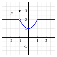
The possible function \(p\) is defined piecewise in the following way: for \(x \lt 1\) and \(x \gt 1\text{,}\) the function is constant with \(p(x) = 1\text{;}\) for \(-1 \lt x \le 1\text{,}\)\(p(x) = x^2 + 1\text{;}\) and \(p(-1) = 3\text{.}\) On the graph, there’s an open circle at \((-1,2)\) and a filled circle at \((-1,3)\text{.}\)
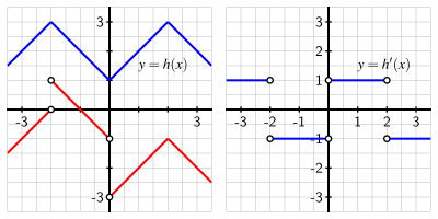
At left, two possible graphs for \(h\text{.}\) The first is shown in blue, and this graph is continuous and piecewise linear. The graph connects the following points using straight lines: \((-3.5,1.5)\) and \((-2,3)\text{;}\)\((-2,3)\) and \((0,1)\text{;}\)\((0,1)\) and \((2,3)\text{;}\) and \((2,3)\) and \((3.5,1.5)\text{.}\) The second possible graph is shown in red, and this graph is also piecewise linear but not continuous. This graph connects the following points using straight lines: \((-3.5,-1.5)\) and \((-2,0)\text{;}\)\((-2,1)\) and \((0,-1)\text{;}\)\((0,-3)\) and \((2,-1)\text{;}\) and \((2,-1)\) and \((3.5,-2.5)\text{.}\) There are open circles at \((-2,0)\text{,}\)\((-2,1)\text{,}\)\((0,-1)\text{,}\) and \((0,-3)\text{.}\)
At right, the given graph of \(y = h'(x)\text{,}\) which is a piecewise constant function whose value is \(1\) for \(x \lt -2\) and \(0 \lt x \lt 2\text{,}\) and whose value is \(-1\) for \(-2 \lt x \lt 0\) and \(x \gt 2\text{.}\) Note that \(h'(x)\) is not defined at \(x = -2, 0, 2\text{,}\) and this is reflected by the open circles at the endpoints of each piece of the graph.
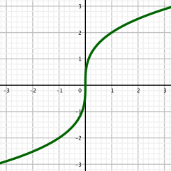
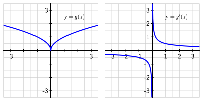
At left, the graph of \(g(x) = \sqrt{|x|}\text{.}\) The graph consists of two pieces of parabolas that open horizontally: for \(x \gt 0\text{,}\) we have the top half of the parabola \(x = y^2\text{;}\) for \(x \lt 0\text{,}\) we have the top half of the parabola \(x = -y^2\text{.}\) Notice that this leads to a sharp corner at the point \((0,0)\) on the graph of \(g\text{.}\)
At right, the graph of \(g'(x)\text{,}\) which appears to be a rational function with a horizontal asymptote of \(y = 0\) and a vertical asymptote at \(x = 0\text{.}\) The graph of \(g'\) looks similar to that of \(y = \frac{1}{x}\) (though that is not the formula for \(g'(x)\)).
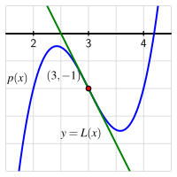
This function appears to be a cubic polynomial that is concave down for \(x \lt 3\) and concave up for \(x \gt 3\text{;}\) its graph passes through the point \((3,-1)\) and the corresponding tangent line does as well, with the tangent line above the graph of \(y = p(x)\) for \(x \lt 1\) and below the graph for \(x \gt 1\text{.}\)
Since \(a^x\) does not depend at all on \(h\text{,}\) we may treat \(a^x\) as constant in the noted limit and thus write the value \(a^x\) in front of the limit being taken.
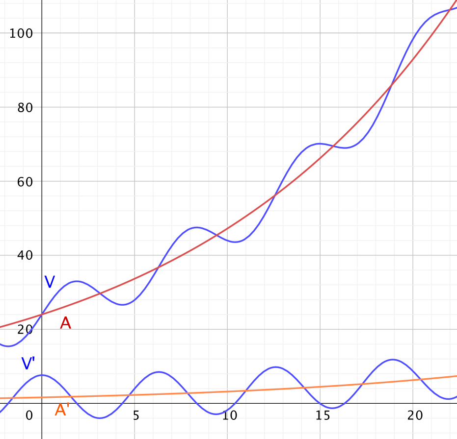
\(V''(2) = 24 \cdot 1.07^2 \cdot \ln(1.07)^2 - 6 \sin(2) \approx -5.33\) thousands of dollars per year per year. At this moment, \(V'\) is decreasing and we expect the derivative’s value to decrease by about \(5.33\) thousand dollars per year over the course of the next year.
The graphs of \(A(t) = 24 \cdot 1.07^t\) and \(V(t) = 24 \cdot 1.07^t + 6 \sin(t)\text{,}\) as well as their derivatives \(A'(t) = 24 \ln(1.07) 1.07^t\) and \(V'(t) = 24 \ln(1.07) 1.07^t + 6 \cos(t)\text{.}\)
Since \(Y(x) = q(q(x))\text{,}\) the chain rule implies that \(Y'(x) = q'(q(x)) \cdot q'(x)\text{,}\) and thus \(Y'(-2) = q'(q(-2)) \cdot q'(-2) = q'(-1) \cdot q'(-2)\text{.}\) But \(q'(-1)\) does not exist, so \(Y'(-2)\) also fails to exist. Using \(Z(x) = q(p(x))\) and the chain rule, we have \(Z'(x) = q'(p(x)) \cdot p'(x)\text{.}\) Therefore \(Z'(0) = q'(p(0)) \cdot p'(0) = q'(-0.5) \cdot p'(0) = 0 \cdot 0.5 = 0\text{.}\)
In (a) we are determining the instantaneous rate at which the volume changes as we increase the height of the water in the tank, while in (c) we are finding the instantaneous rate at which volume changes as we increase time.
Consider \(\lim_{x \to \infty} \frac{p(x)}{e^x} \) By repeated application of LHR, the numerator will eventually be simply a constant (after \(n\) applications of LHR), and thus with \(e^x\) still in the denominator, the overall limit will be \(0\text{.}\)
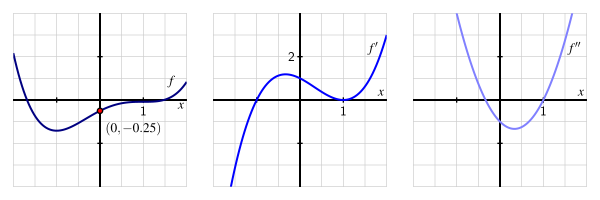
\(f'\) is positive for \(-1 \lt x lt 1\) and for \(x \gt 1\text{;}\)\(f'\) is negative for all \(x \lt -1\text{.}\)\(f\) has a local minimum at \(x = -1\text{.}\)
\(f''(x)\) is negative for \(-0.35 \lt x \lt 1\text{;}\)\(f''(x)\) is positive everywhere else; \(f\) has points of inflection at \(x \approx -0.35\) and \(x = 1\text{.}\)
\(g\) does not have a global minimum; it is unclear (at this point in our work) if \(g\) increases without bound, so we can’t say for certain whether or not \(g\) has a global maximum.
\(p''(x)\) is negative for \(-1 \lt x \lt 2\) and positive for all other values of \(x\text{;}\)\(p\) has points of inflection at \(x = -1\) and \(x = 2\text{.}\)
Absolute max \(s(\frac{5\pi}{12}) = 8\text{;}\) absolute min \(s(\frac{11\pi}{12}) = 2\text{.}\) (There are other points at which the function achieves these values on the given interval.)
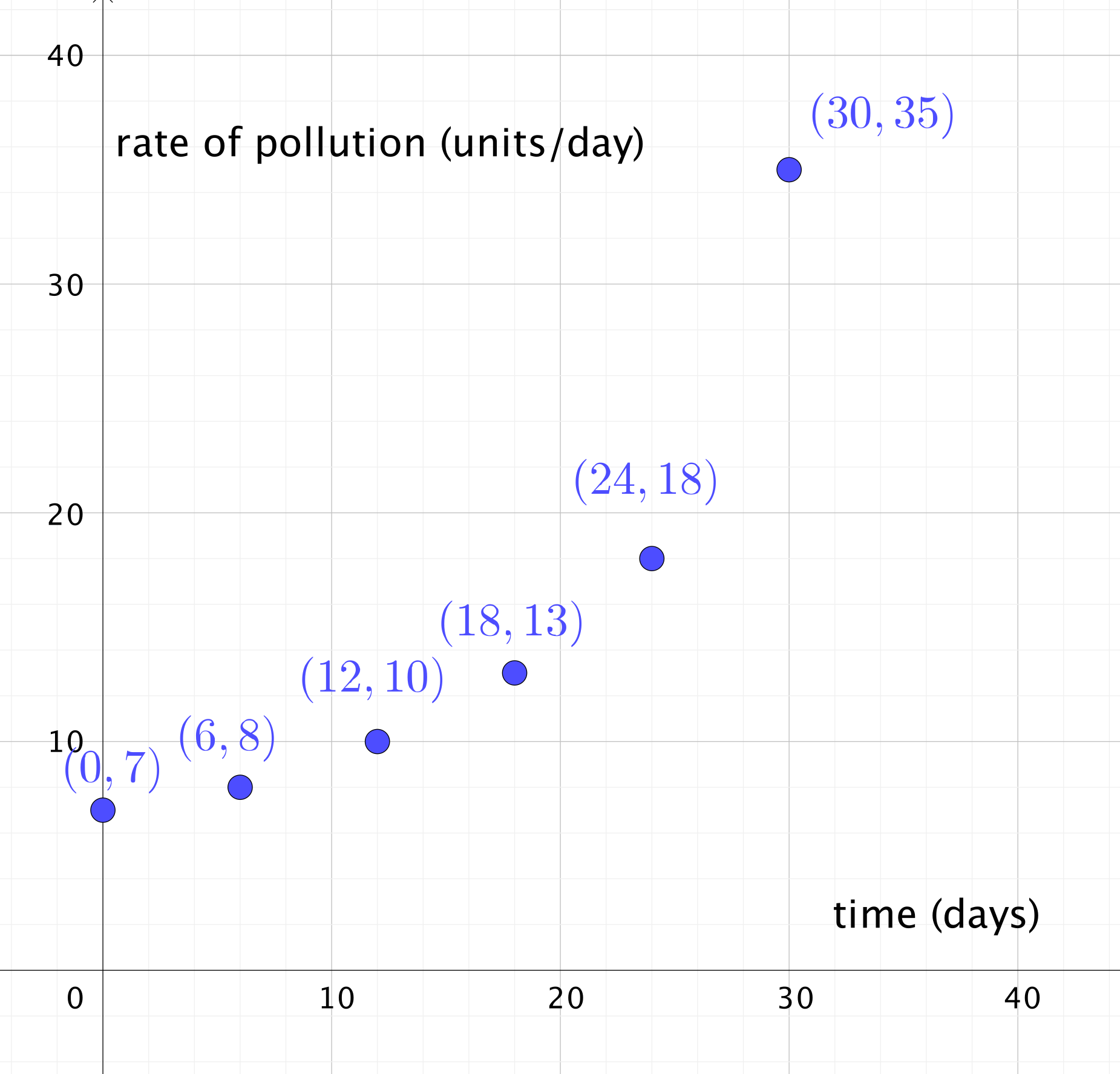
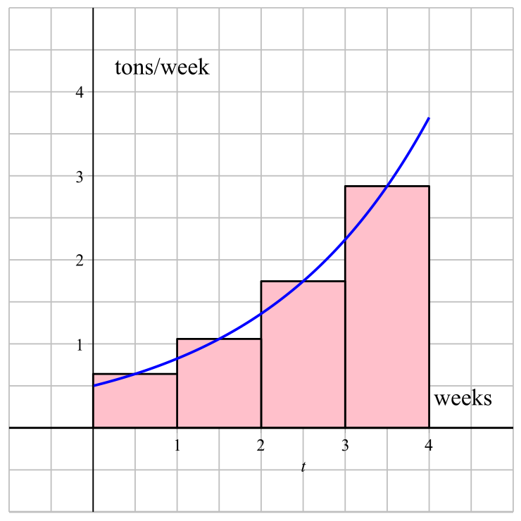
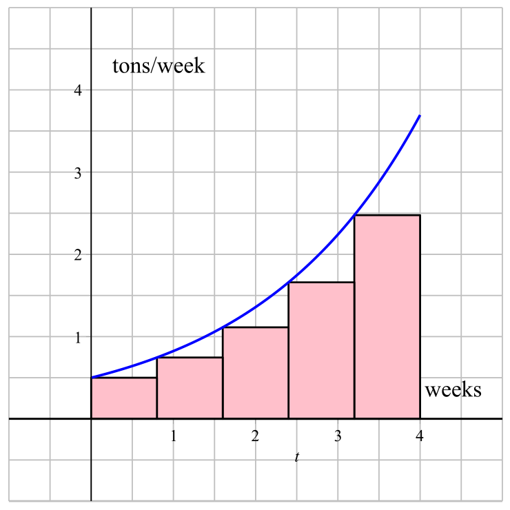
Think about the product of the units involved: “units of pollution per day” times “days”. Connect this to the area of a thin vertical rectangle whose height is given by the curve.
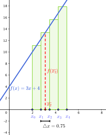
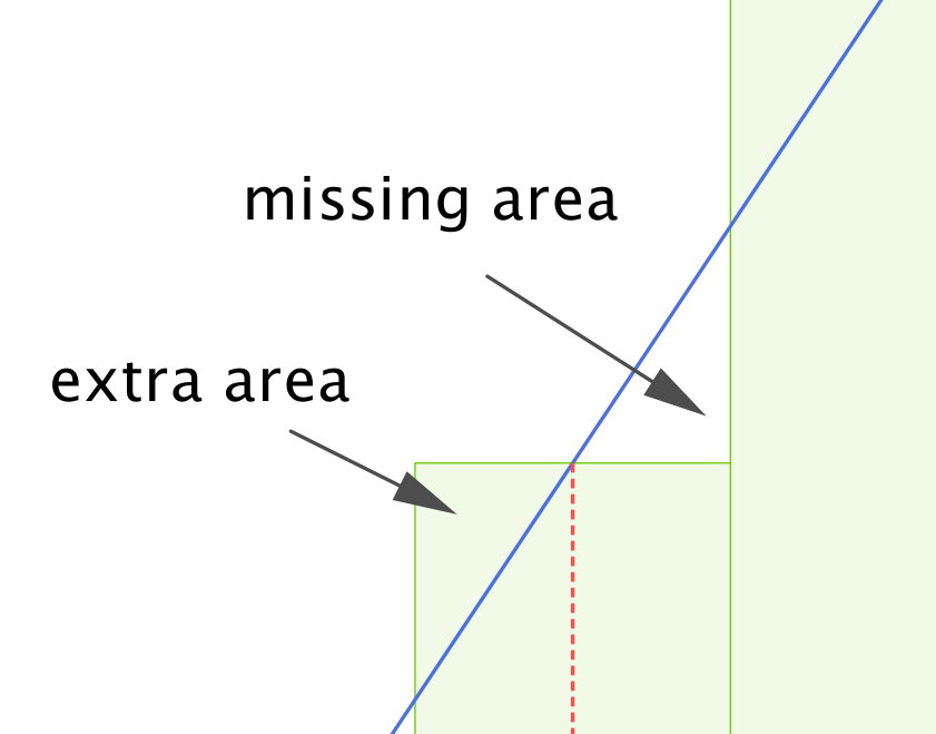
The rectangles with heights that come from the midpoint have the same area as the trapezoids that are formed by the function values at the two endpoints of each subinterval.
If \(S\) is a left Riemann sum, \(f(x) = x^2 + 1\) on the interval \([1.4, 3.4]\text{.}\) If \(S\) is a middle Riemann sum, \(f(x) = x^2 + 1\) on the interval \([1.2, 3.2]\text{.}\)
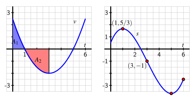
Two sets of adjacent coordinate axes are provided, both showing the independent variable ranging horizontally from \(-0.5\) to \(6.5\) and the dependent variable ranging vertically from \(-3.5\) to \(3.5\text{.}\) The grid is \(0.5 \times 10.5\text{.}\)
At right, the position function \(y = s(t)\) is shown. The function \(s(t)\) is a cubic function that passes through the following important points: \((0,0.5)\text{,}\)\((1,5/3)\text{,}\)\((3,-1)\text{,}\)\((5,-11/3)\text{,}\) and \((6,-2.5)\text{.}\) We note that \(s(t)\) is increasing for \(0 \lt t \lt 1\) and for \(5 \lt t \lt 6\text{,}\) and decreasing for \(1 \lt t \lt 5\text{;}\) in addition, \(s(t)\) is concave down for \(0 \lt t \lt 3\) and concave up for \(3 \lt t \lt 6\text{.}\)
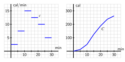
Two sets of adjacent coordinate axes are provided, both showing the independent variable ranging horizontally from \(-5\) to \(35\text{.}\) On the left grid,the dependent variable ranges vertically from \(-2.5\) to \(17.5\text{.}\) On the left grid, the vertical scale is \(-50\) to \(350\text{.}\)
At right, the piecewise linear (and continuous) function \(y = C(t)\) is plotted. The graph shows how \(y = C(t)\) passes through each of the points identified in the preceding question(s) (e.g., \(C(15)=125\)), and the graph of \(C(t)\) has a corner point at each location where there is a jump in the value of its derivative \(c(t)\text{.}\)
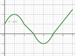
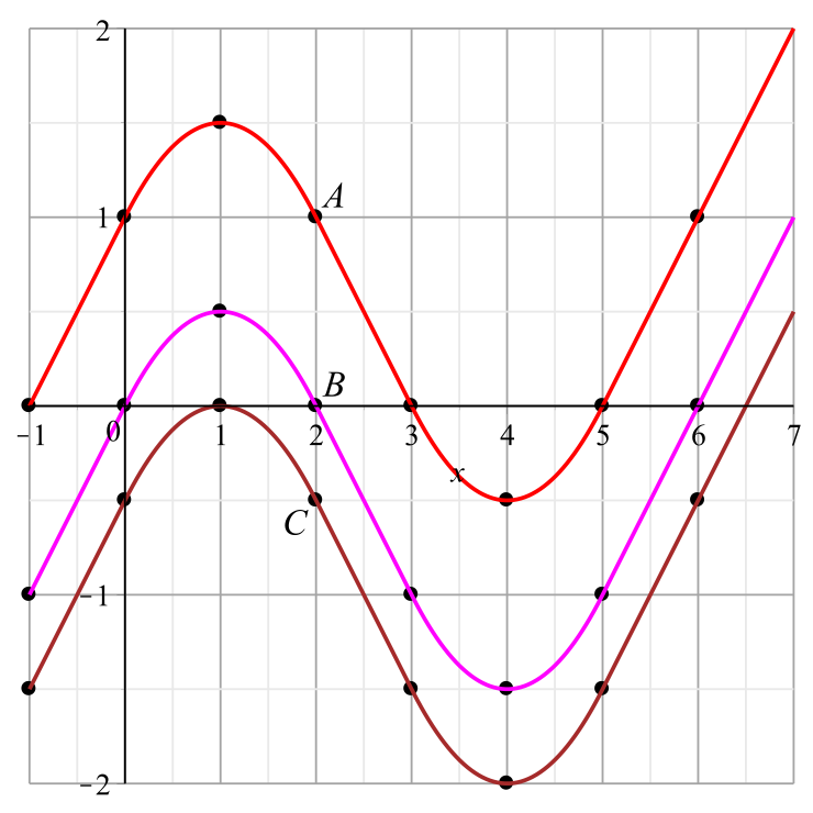
Two sets of adjacent coordinate axes are provided, both showing the independent variable ranging horizontally from \(-1\) to \(7\) and \(y\) ranging vertically from \(-4\) to \(4\text{.}\) The grid is \(1 \times 1\text{.}\)
At right, the functions \(A(x)\text{,}\)\(B(x)\text{,}\) and \(C(x)\) are shown. The function \(A(x)\) satisfies all of the values determined in the preceding question(s) (e.g., \(A(1)=1.5\)). The graph of \(A(x)\) is linear on the intervals where \(f(t)\) is constant, and on those intervals the slope of \(A(x)\) matches the value of \(f(t)\text{.}\) For example, on \(2 \lt x \lt 3\text{,}\)\(A(x)\) is linear with slope \(-1\text{.}\) The graph of \(A(x)\) is linear on the intervals where \(f(t)\) is linear with nonzero slope. For example, on \(3 \lt x \lt 5\text{,}\)\(A(x)\) is a concave up parabola.
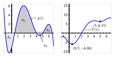
\(F\) is increasing on \(x \lt -1\text{,}\)\(0.5 \lt x \lt 4\text{,}\) and \(5 \lt x \lt 6.5\text{;}\) decreasing on \(-1 \lt x \lt 0.5\) and \(4 \lt x \lt 5\text{;}\) concave up on approximately \(-0.4 \lt x \lt 2\) and \(4.5 \lt x \lt 6\text{;}\) concave down on approximately \(2 \lt x \lt 4.5\) and \(x \gt 6\text{;}\)\(F(2) = 0\text{;}\)\(F(0.5) = -6.06\text{;}\)\(F(-1) = -1.77\text{;}\)\(F(4) = 6.69\text{;}\)\(F(5) = 6.33\text{;}\)\(F(6.5) = 8.12\text{.}\)
There are two adjacent graphs, both shown on the horizontal interval from \(-1.5\) to \(7\text{.}\) The vertical scale on the left axes is \(-4.5\) to \(6.5\text{.}\) The vertical scale on the right axes is \(-11\) to \(16\text{.}\) The righthand plot is where the solution to this exercise is plotted.
At left, the given graph of \(y = g(t)\text{.}\) The function \(y = g(t)\) is a degree \(5\) polynomial that has zeros at \(x = -1, 0.5, 4, 5, 6.5\text{;}\) the function is negative on the interval \(-1 \lt x \lt 0.5\) and changes sign at each of its zeros. In addition, each of the four finite regions that \(g(t)\) bounds with the \(t\)-axis are shaded and labeled from left to right: \(A_1\text{,}\)\(A_2\text{,}\)\(A_3\text{,}\) and \(A_4\text{.}\) For example, \(A_2\) is the region between the second pair of adjacent zeros, from \(x = 0.5\) to \(x = 4\text{.}\)
At right, a graph of the function \(F(x) = \int_{2}^x g(t) \, dt\text{.}\) This curve has the described properties and values that have been noted in the preceding parts of this exercise. Two key points are shown and labeled on the graph of \(F\text{:}\)\((0.5, -6.06)\) and \((5, 6.33)\text{.}\)
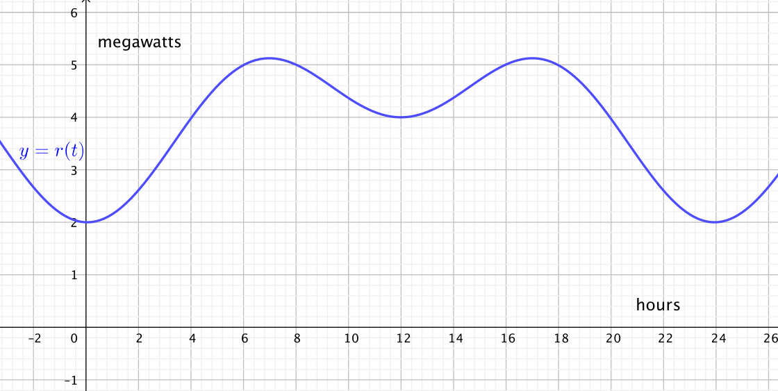
The model is reasonable because it appears to be periodic and the rate of consumption seems to peak at the times of day where people are most active in their homes.
A plot of \(r(t) = 4 + \sin(0.263t + 4.7) + \cos(0.526t+9.4)\) on the interval \(-2 \lt t \lt 26\text{.}\) The function has equal global minimums at \(t = 0\) and \(t = 24\text{,}\) equal global maxnimums at \(t \approx 7\) and \(t \approx 17\text{,}\) and a local minimum at \(t = 12\text{.}\)
\(u\)-substitution fails since there’s not a composite function present; try showing that each of the choices of \(u = x\) and \(dv = \tan(x) \, dx\text{,}\) or \(u = \tan(x)\) and \(dv = x \, dx\text{,}\) fail to produce an integral that can be evaluated by parts.
\(\frac{1}{60} S_6 \approx 3438.89
\text{;}\)\(\frac{2000+2100+2400+3000+3900+5100+6500}{7} = \frac{25000}{7} \approx 3571.43
\text{.}\) each estimates the average rate at which water flows through the dam on \([0,60]\text{,}\) and the first is more accurate.
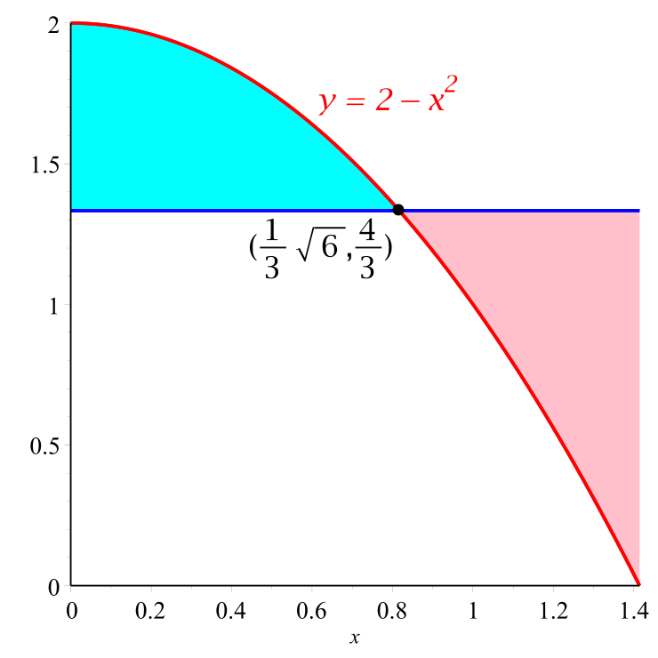
A plot of \(f(x) = 2-x^2\) on the interval \([0,\sqrt{2}]\text{,}\) along with its average value on the interval, \(y = \frac{4}{3}\text{.}\) The function \(f\) lies above its average value for \(0 \lt x \lt \frac{\sqrt{6}}{3}\) and below its average value for the remainder of the interval up to \([\sqrt{2}]\text{.}\)
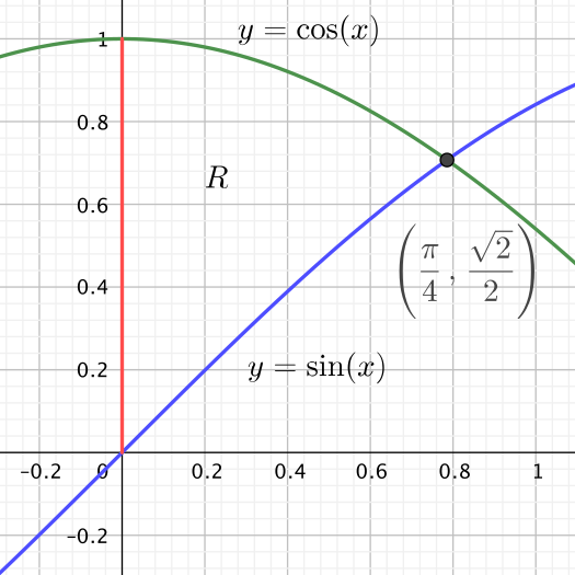
This figure shows the functions \(y = \cos(x)\) and \(y = \sin(x)\) plotted on the interval \([0,1]\) with the region \(R\) they bound along with the \(y\)-axis on the interval \([0, \frac{\pi}{4}]\) (the two curves intersect at the point (\frac{\pi}{4}, \frac{\sqrt{2}}{2}), which is shown and labeled).
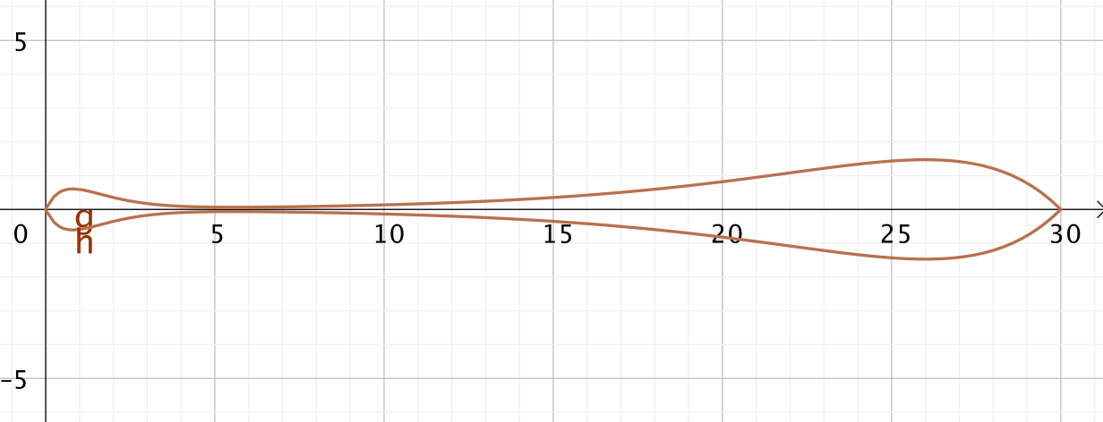
This plot shows the function \(y = f(x) = 2xe^{-1.25x} + (30-x) e^{-0.25(30-x)}\) on the interval \([0,30]\) and its reflection across the \(x\)-axis to form the described solid of revolution.
At a given \(x\)-location, the amount of weight concentrated there is approximately the weight density (\(0.6\) ounces per cubic inch) times the volume of the slice, which is \(V_{text{slice}} \approx \pi f(x)^2\text{.}\)
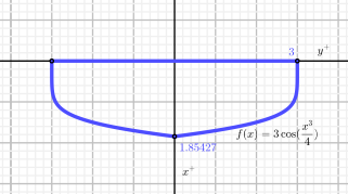
The coordinate axes are oriented \(90^{\degrees}\) clockwise from what is typical so that the positive \(y\)-axis points to the right and the positive \(x\)-axis points down. In the first quadrant, the function \(f(x) = 3 \cos(\frac{x^3}{4})\) is plotted with two key points labeled: \((0,3)\) and \((1.85427,0)\text{.}\) The region the function bounds in the first quadrant is then reflected across the positive \(x\)-axis to show one end of the described tank, which looks something like the cross section of the hull of a boat.
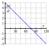
\(\frac{dT}{dt}\vert_{T=105} = -2\text{;}\) when \(T = 105\text{,}\) the coffee’s temperature is decreasing at an instantaneous rate of \(-2\) degrees F per minute.
A plot of \(\frac{dT}{dt}\) as a function of \(T\) using the differential equation \(\frac{dT}{dt}= -\frac1{15}T+5\text{.}\) The values of \(T\) range horizontally from \(T=0\) to \(T=120\text{,}\) and the values of \(\frac{dT}{dt}\) range vertically from \(\frac{dT}{dt}=-3\) to \(\frac{dT}{dt}=5\text{.}\) The graph is a straight line that passes through \((75,0)\) with a slope of \(m=-1/15\text{.}\)
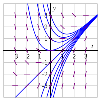
Along the line \(y = t-1\text{,}\) every line segment in the slope field has slope \(m=1\text{,}\) and along the line \(y = t\text{,}\) every line segment has slope \(m=0\text{.}\) Below the line \(y = t-1\text{,}\) every line segment has positive slope greater than \(1\text{,}\) and above the line \(y = t\text{,}\) every line segment has negative slope.
When we plot solution curves, there’s a straight line solution that satisfies \(y = t-1\) (this solution satisfies \(y(0) = -1\)). For solutions with \(y(0) \lt -1\text{,}\) the solution is always increasing and concave down, plus it tends toward the line \(y = t-1\) as \(t\) increases without bound. For solutions with \(y(0) \gt -1\text{,}\) the solution is decreasing for \(t\) values up to where the curve crosses the line \(y = t\text{,}\) and then increasing for \(t\) values thereafter; such a solution is always concave up, and also tends toward the line \(y = t-1\) as \(t\) increases without bound.
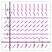
The slope field for the differential equation \(\frac{dP}{dt}=f(P)\text{.}\) Because the differential equation is autonomous, the slopes of segments in the slope field only depend on \(P\) and not on \(t\text{;}\) that is, along any horizontal line, the slopes will all have the same value.
The slope field has three horizontal lines where the slope of every line segment is zero: \(P=0\text{,}\)\(P=1\text{,}\) and \(P=3\text{.}\) For \(P\) values that satisfy \(P \gt 3\) or \(0 \lt P \lt 1\text{,}\) the slopes are all negative. For \(P\) values that satisfy \(1 \lt P \lt 3\) or \(P \lt 0\text{,}\) the slopes are all positive.
Any solution curve that starts with \(P(0) \gt 3\) will decrease to \(P(t) = 3\) as \(t \to \infty\text{;}\) any curve that starts with \(1 \lt P(0) \lt 3\) will increase to \(P(t) = 3\text{;}\) any curve that starts with \(0 \lt P(0) \lt 1\) will decrease to \(P(t) = 0\text{.}\)
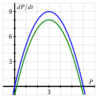
The graph of \(f(P) = P(6-P)\) is a concave down parabola with vertex at \(P = 3\) and zeros at \(P = 0\) and \(P = 6\text{.}\) The graph of the updated function \(g(P) = P(6-P)-1\) is the original curve just shifted down \(1\) unit, which leads to the second function having zeros slightly larger than \(P = 0\) (at about \(P \approx 0.172\)) and slightly smaller than \(P = 6\) (at about \(P \approx 5.83\)).
If \(P \lt \frac{6-\sqrt{32}}{2}\text{,}\) then the fish population will die out. If \(\frac{6-\sqrt{32}}{2} \lt P\text{,}\) then the fish population will approach \(\frac{6+\sqrt{32}}{2}\) thousand fish.
For positive \(y\) near \(0\text{,}\)\(M(y) = \frac{y}{2+y} \approx 0\text{;}\) for large values of \(y\text{,}\)\(M(y) = \frac{y}{2+y} \approx 1\text{.}\)
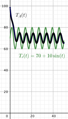
This plot superimposes the graph of the forcing function, \(T_r(t) = 70+ 10\sin(t)\) with the \(500\) data points that result from using Euler’s Method to approximate the solution to the IVP that corresponds to Alice’s coffee, \(T_A(t)\text{.}\) The plot is shown in the window where \(0 \le t \le 50\) and \(0 \le T \le 110\text{.}\)
The forcing function \(T_r(t)\) oscillates between \(60\) and \(80\) degrees, and this makes \(T_A(t)\) eventually oscillate with a similar frequency but with a smaller amplitude, varying between approximately \(65\) and \(75\) degrees. The solution function \(T_A(t)\) starts at \(T_A(0) = 100\) and then decreases quickly to about \(65\) degrees around \(t = 5\text{,}\) and then oscillates as previously described.
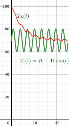
This plot superimposes the graph of the forcing function, \(T_r(t) = 70+ 10\sin(t)\) with the \(500\) data points that result from using Euler’s Method to approximate the solution to the IVP that corresponds to Bob’s coffee, \(T_B(t)\text{.}\) The plot is shown in the window where \(0 \le t \le 50\) and \(0 \le T \le 110\text{.}\)
The forcing function \(T_r(t)\) oscillates between \(60\) and \(80\) degrees, and this makes \(T_B(t)\) eventually oscillate with a similar frequency but here with a much smaller amplitude, varying between approximately \(70\) and \(72\) degrees. The solution function \(T_B(t)\) starts at \(T_B(0) = 100\) and then decreases fairly slowly (with slight oscillations) to about \(70\) degrees around \(t = 44\text{,}\) and then oscillates as previously described.
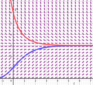
The most prominent feature of the slope field is the equilibrium solution shown at \(P = 3\text{.}\) Slopes are constant for any fixed value of \(P\) for every value of \(t\text{.}\) When \(P \gt 3\text{,}\) slopes are negative, and more negative the further \(P\) is from \(3\text{.}\) When \(0 \lt P \lt 3\text{,}\) slopes are positive, and most positive around \(P \approx 1.1\text{.}\) negative the further \(P\) is from \(3\text{.}\) The figure also shows two solutions: one that satisfies \(P(0) = 5\) that is always decreasing and approaches \(P=3\text{,}\) and the other satisfies \(P(0) = 1\) and is always decreasing and also approaches \(P=3\text{.}\)
\(T_6(x)\) appears to be the same as \(P_6(x-\frac{\pi}{2})\text{,}\) the degree \(6\) Taylor polynomial of \(\cos(x)\) centered at \(a = 0\text{,}\) shifted \(\frac{\pi}{2}\) units to the right.
Since \(\sin(x) = \cos(x - \frac{\pi}{2})\text{,}\) this tells us that the sine function is simply a shifted version of the cosine function (the cosine function shifted \(\frac{\pi}{2}\) units to the right).